How to Freeze Panes in Excel Both Horizontally and Vertically

PlanetNumber1

Editor

posted on 2 years ago — updated on 1 second ago

17
views

This wikiHow will show you how to freeze panes in Excel to show horizontal and vertical rows and columns at the same time. When you freeze a column or a row, it will stay visible when you're scrolling through that worksheet.

Things You Should Know

To start, you need to select a cell to the right of the column and below the row you want to freeze.
You can freeze panes by going to the View tab on the ribbon and selecting the Freeze Panes button.
This method works on Excel for Office 365, Excel for the web, Excel 2019, Excel 2016, Excel 2013, Excel 2010, Excel 2007 for Windows and Mac.

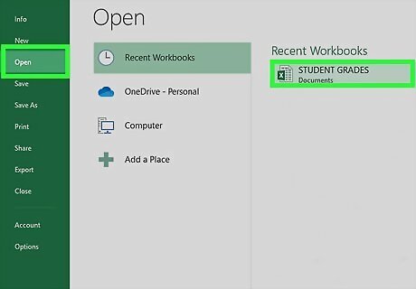
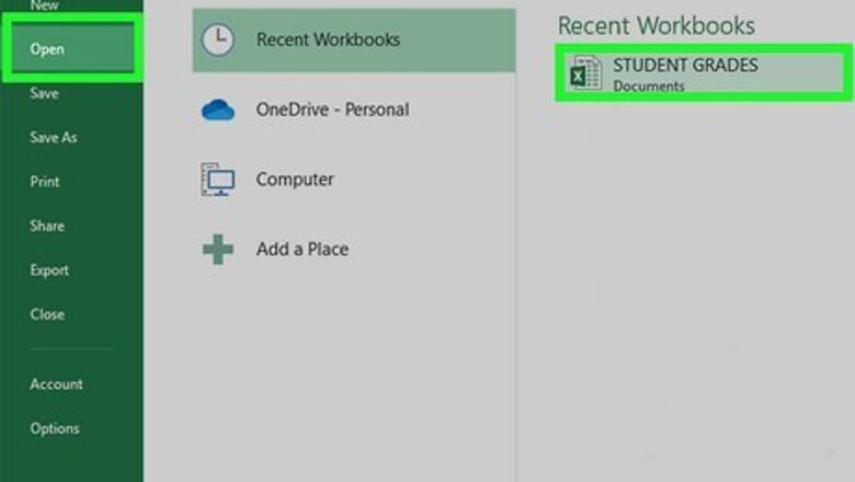
Open your project in Excel. You can either open the program within Excel by clicking File > Open, or you can right-click the file in your file explorer. This will work for Windows and Macs using Excel for Office 365, Excel for the web, Excel 2019, Excel 2016, Excel 2013, Excel 2010, Excel 2007.

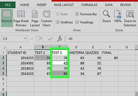
Select a cell to the right of the column and below the row you want to freeze. The frozen columns will remain visible when you scroll through the worksheet.

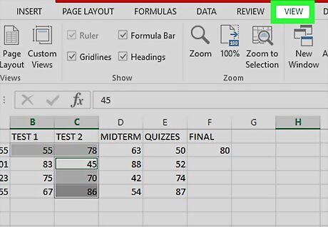
Click View. You'll see this either in the editing ribbon above the document space or at the top of your screen.

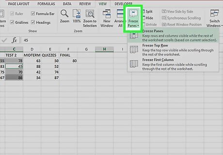
Click Freeze Panes. A menu will dropdown.

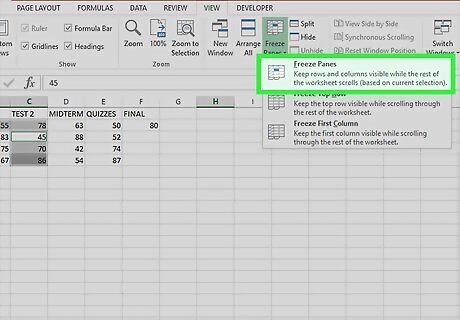
Click Freeze Panes. This will freeze the panes in the columns next to what you have selected. Unfreeze columns by going to View > Freeze Panes > Unfreeze Panes.