
Previous Lessons Learned
Be sure that you have done the three previous spreadsheets. They are: Create Artistic Patterns in Microsoft Excel Create a Flower Pattern in Microsoft Excel Create a Tornado Screw Pattern in Microsoft Excel
Complete those first before attempting this one because there was a sequence to building the worksheets.
The Tutorial
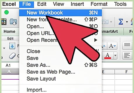
Start a new workbook by saving the old workbook under a new name. Save the workbook into a logical file folder.
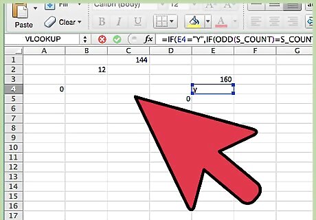
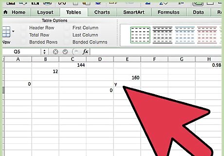
Set variables to various values and set formulas correctly. Set A4, On=0,Off=1, to 0. Set B2, TURNS, to 12. Set C1, S's Count, to 144. Set D5, AAA, to 0. Set E3, Divisor to 160. Set H1 to .98 and J1 to .96 Set E4, YN, to Y. The formula in Factor is "=IF(E4="Y",IF(ODD(S_COUNT)=S_COUNT,-S_COUNT*0.01,S_COUNT*0.01),-0.25)" Adjuster is set to 1 and AdjRows to 1439. t is -308100. Adj is "=IF(TURNS>0,VLOOKUP(TURNS,TURNS_LOOKUP,2),VLOOKUP(TURNS, TURNS_LOOKUP_NEG,2))" Designer is "=VLOOKUP(S_COUNT,SPHEROIDS_COUNT_LOOKER,2)" Var is "=IF(S_COUNT<4,S_COUNT+30,12)" Cc is "=-0.25*PI()/C3" db is 4.5 top is "=ROUND((-B4*PI())+(Adj),0)" 968,277 H2 is Sync1 "=H1/GMLL" J2 is Sync2 "=J1/GMSL"
None of the Lookup tables have changed.
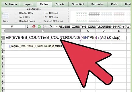
The column formulas are as follows: B7: "=IF(EVEN(S_COUNT)=S_COUNT,ROUND((-B4*PI())+(Adj),0),top)" B8;B1447: "=((B7+(-TOP*2)/(AdjRows)))*$B$1" C7: "=ROUND(-EXP((PI()^2)+(Cc*-(db))),0)+Designer" C8:C1447: "=C7" D7:D1447: "=IF(A7=0,D6,DEGREES((ROW()-7))*COS((ROW()-7)*Factor*PI()/(180))/Divisor)" which looks new. E7:E1447: "=IF(A7=0,E6,DEGREES((ROW()-7))*SIN((ROW()-7)*Factor*PI()/(180))/Divisor)" F7:F1447: "=IF(A7=0,F6,((PI())*((SIN(B7/(C7*2))*GMLL*COS(B7)*GMLL*(COS(B7/(C7*2)))*GMLL)+D7)))" G7:G1447: "=IF(A7=0,G6,((PI())*((SIN(B7/(C7*2))*GMLL*SIN(B7)*GMLL*(COS(B7/(C7*2)))*GMLL)+E7)))" H7:H1447: "=F7*GMLL*Sync1" I7:I1447: "=G7*GMLL*Sync1" J7:J1447: "=F7*GMSL*Sync2" K7:K1447: "=G7*GMSL*Sync2" A7:A1447: (without spaces) "=IF(OR(AND((ROW()-7)>Rrs,(ROW()-7)<=Rrs*2),AND((ROW()-7)>Rrs*4,(ROW()-7)<=Rrs*5), AND((ROW()-7)>Rrs*7,(ROW()-7)<=Rrs*8), AND((ROW()-7)>Rrs*10,(ROW()-7<=Rrs*11),AND((ROW()-7)>Rrs*13,(ROW()-7<=Rrs*14), AND((ROW()-7)>Rrs*16,(ROW()-7<=Rrs*17), AND((ROW()-7)>Rrs*19,(ROW()-7)<=Rrs*20), AND((ROW()-7)>Rrs*22,(ROW()-7<=Rrs*23), AND((ROW()-7)>Rrs*25,(ROW()-7)<=Rrs*26), AND((ROW()-7)>Rrs*28,(ROW()-7)<=Rrs*29), AND((ROW()-7)>Rrs*31,(ROW()-7)<=Rrs*32), AND((ROW()-7)>Rrs*34,(ROW()-7)<=Rrs*35), AND((ROW()-7)>Rrs*37,(ROW()-7)<=Rrs*38), AND((ROW()-7)>Rrs*40,(ROW()-7)<=Rrs*41)),0,1)+On_0_Off_1
Explanatory Charts, Diagrams, Photos
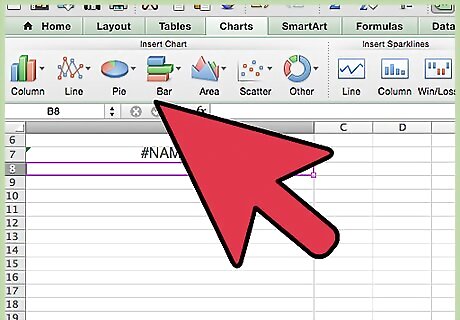
Create the charts. These flow from F7:G1446, H7:I1446 and J7:K1446, the latter two being copied in or Added Series independently and corrections made until the series look like this: =SERIES(,'CosSin to Base X,Y DATA'!$H$7:$H$1446,'CosSin to Base X,Y DATA'!$I$7:$I$1446,1) in ice blue or green-blue, it's hard to tell. Line weight is .25 for all. =SERIES(,'CosSin to Base X,Y DATA'!$J$7:$J$1446,'CosSin to Base X,Y DATA'!$K$7:$K$1446,2) in red-lavender =SERIES(,'CosSin to Base X,Y DATA'!$F$7:$F$1446,'CosSin to Base X,Y DATA'!$G$7:$G$1446,3) in blue
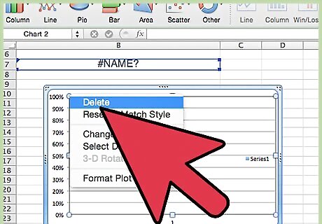
Remove Axis, Grid lines and Chart Legend for both charts in Chart Layout.


Comments
0 comment