
- Freeze a row by going to View > Freeze Panes.
- Print a row across multiple pages using Page Layout > Print Titles.
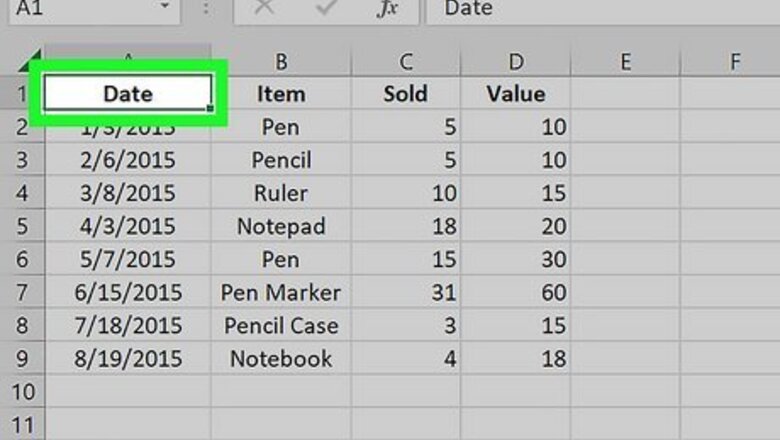
- Create a table with headers with Insert > Table. Select My table has headers.
- Add headers to a Power Query table: Query > Edit > Transform > Use First Row as Headers.
Keeping the Header Row Visible
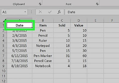
Select a cell in the row you want to freeze. You can set Excel to freeze your header row so it's always visible, even as you scroll. If your header row is in row 1, you don't have to click any cells. Just continue to the next step. If your header row is down further, such as in row 2 or 3, click a cell below the header row. For example, if the row that contains your column labels is row 5, you will need to click a cell in row 6.
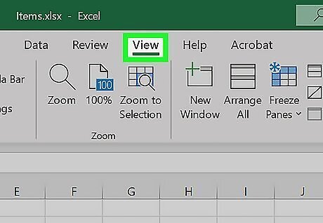
Click the View tab. You'll see it at the top of the window.
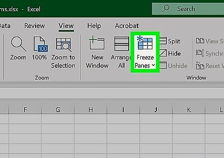
Click Freeze Panes. This menu is in the toolbar at the top of Excel. A list of freezing options will appear.
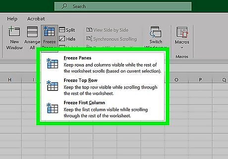
Select a Freeze Pane option. The option you select on this menu depends on whether your header row is in row 1 or in a different row: If your header row is in row 1 (the first row on your sheet), select Freeze Top Row. This ensures that the top row of your sheet remains locked into position, even as you scroll through your data. If your header row is in a different row, such as row 3, select Freeze Panes. This freezes the row above the cell you selected in Step 1. For example, if you selected A6 in Step 1, selecting Freeze Panes will freeze row 5, making it your header row. This row will always stay visible as you scroll through your data. The Freeze Panes option works as a toggle. That is, if you already have panes frozen, clicking the option again will unfreeze your current setup. Clicking it a second time will refreeze the panes in the new position.
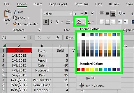
Add emphasis to your header row (optional). Create a visual contrast for this row by centering the text in these cells, applying bold text, adding a background color, or drawing a border under the cells. this can help the reader take notice of the header when reading the data on the sheet.
Printing a Header Row Across Multiple Pages
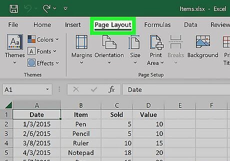
Click the Page Layout tab. If you have a large worksheet that spans multiple pages that you need to print, you can set a row or rows to print at the top of every page.
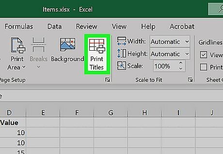
Click the Print Titles button. You'll find this in the Page Setup section.
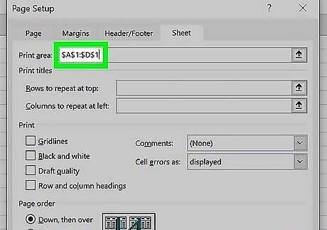
Set your Print Area to the cells containing the data. Click the button next to the Print Area field and then drag the selection over the data you want to print. Don't include the column headers or row labels in this selection.
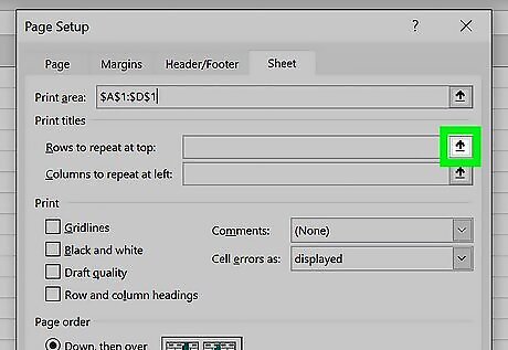
Click the button next to "Rows to repeat at top." This will allow you to select the row(s) that you want to treat as the constant header.
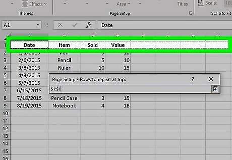
Select the row(s) that you want to turn into a header. The rows that you select will appear at the top of every printed page. This is great for keeping large spreadsheets readable across multiple pages.
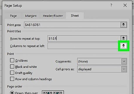
Click the button next to "Columns to repeat at left." This will allow you to select columns that you want to keep constant on each page. These columns will act like the rows you selected in the previous step, and will appear on every printed page.
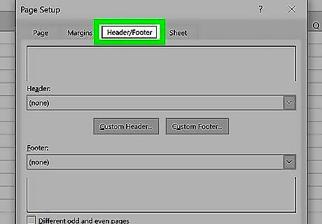
Set a header or footer (optional). You can include the company title or document title at the top, and insert page numbers at the bottom. This will help the reader get the pages organized. To set the header and footer: Click the Header/Footer tab Click the Header or Footer drop down menus to select a preset header. Alternatively, click Custom Header or Custom Footer to create your own.
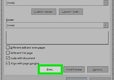
Print your sheet. You can send the spreadsheet to print now, and Excel will print the data that you set with the constant header and columns you chose in the Print Titles window. Click Print to start the printing process. Check the print preview in the preview section. Click Print (the printer icon) to print the spreadsheet.
Creating a Header in a Table
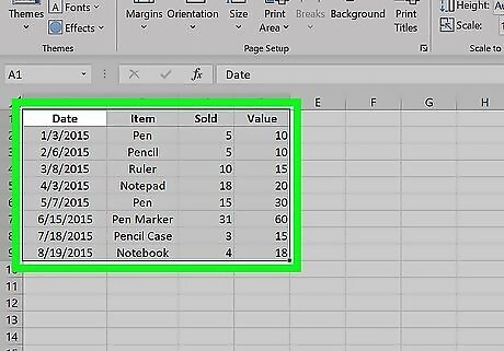
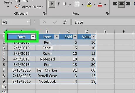
Select the data that you want to turn into a table. When you convert your data to a table, you can use the table to manipulate the data. One of the features of a table is the ability to set headers for the columns. Note that these are not the same as worksheet column headings or printed headers. For example, if you’re using Excel to track your bills, you might have headers like Date, Expense Type, and Amount.
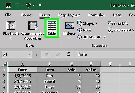
Click the Insert tab and click Table. Confirm that your selection is correct. If you’re looking for Pivot Table information, check out our intro guide here.
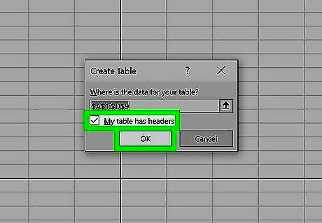
Check the "My table has headers" box and click OK. This will create a table from the selected data. The first row of your selection will automatically be converted into column headers. If you don't select "My table has headers," a header row will be created using default names. You can edit these names by selecting the cell.
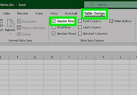
Enable or disable the header. This will show or hide the header. It won’t delete the header information, so you can turn it on and off as needed. Click the Design tab Check or uncheck the "Header Row" box to toggle the header row on and off. You can find this option in the Table Style Options section of the Design tab. Note that turning the header off will also remove any applied filters from the table.
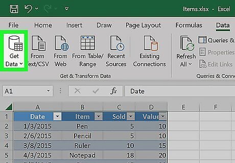
Add and Rename Headers in Power Query
Select a cell in your imported data. This will cause the “Table Design” and “Query” tabs to appear at the top of Excel. This method is used to add row headers to the dataset you imported using Get & Transform (Power Query). You’ll also be able to rename existing headers using this method. Note that this method requires the first row of your dataset to contain column header names.
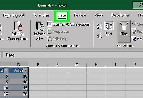
Click Query. This is the rightmost tab at the top of Excel.
Click Edit in the Query tab. This is the icon with a spreadsheet and pencil. The Power Query Editor window will open.
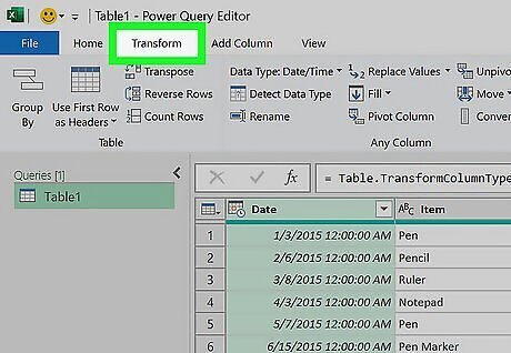
Click Transform. This is a tab at the top of the Power Query Editor.
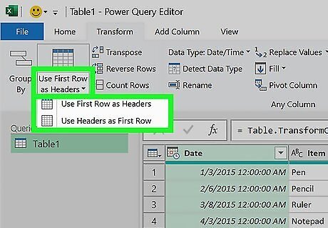
Make the first row of data the header. To do so: Click Use First Row as Headers. Select Use First Row as Headers in the drop down menu. This will make row 1 into the headers for the table.
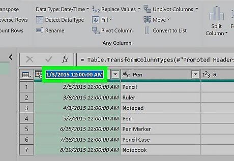
Rename the headers. In the Power Query Editor, you can rename the column headers using these steps: Double-click the column header name. Type in a new name for the header. Press ↵ Enter to confirm the name.
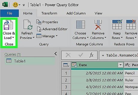
Click Close & Load in the Home tab of the editor. This will reload the imported table with the changes you made in the editor.


Comments
0 comment