How to Calculate Line Integrals

Scalar Fields

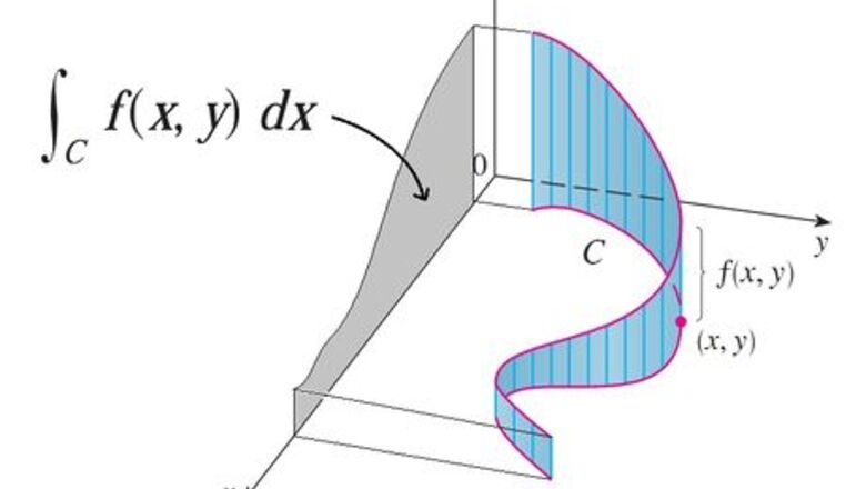
Apply the Riemann sum definition of an integral to line integrals as defined by scalar fields. We want our function f {\displaystyle f} f to be a function of more than one variable, and our differential element d s {\displaystyle \mathrm {d} s} {\mathrm {d}}s must only depend on the curve itself and not the coordinate system we are using. As seen by the diagram above, all we are doing is generalizing the area under a curve as learned in single-variable calculus, whose path is restricted to the x-axis only. This step is not necessary to solve problems dealing with line integrals, but only provides a background to how the formula arises. lim Δ s i → 0 ∑ i = 1 n f ( x i , y i ) Δ s i {\displaystyle \lim _{\Delta s_{i}\to 0}\sum _{i=1}^{n}f(x_{i},y_{i})\Delta s_{i}} \lim _{{\Delta s_{{i}}\to 0}}\sum _{{i=1}}^{{n}}f(x_{{i}},y_{{i}})\Delta s_{{i}} This form should seem familiar to you. We are adding up rectangles with height f ( x i , y i ) {\displaystyle f(x_{i},y_{i})} f(x_{{i}},y_{{i}}) and width Δ s i . {\displaystyle \Delta s_{i}.} \Delta s_{{i}}. These rectangles are bounded by our curve, as recognized by the s {\displaystyle s} s variable, signifying arc length. Then, we take the limit as Δ s i → 0 {\displaystyle \Delta s_{i}\to 0} \Delta s_{{i}}\to 0 to recover the integral, where the Δ s {\displaystyle \Delta s} \Delta s is replaced by the differential d s . {\displaystyle \mathrm {d} s.} {\mathrm {d}}s. Below, C {\displaystyle C} C is the curve over which we are integrating. ∫ C f ( x , y ) d s {\displaystyle \int _{C}f(x,y)\mathrm {d} s} \int _{{C}}f(x,y){\mathrm {d}}s

Reparameterize the integrand in terms of t {\displaystyle t} t. While the integral above is true, it is not very useful, as the calculations can quickly become clunky. Inevitably, we need a coordinate system to work with - one that we can choose for our convenience. Consider the integral ∫ C x y 4 d s , {\displaystyle \int _{C}xy^{4}\mathrm {d} s,} \int _{{C}}xy^{{4}}{\mathrm {d}}s, where C {\displaystyle C} C is the right half of the circle x 2 + y 2 = 16. {\displaystyle x^{2}+y^{2}=16.} x^{{2}}+y^{{2}}=16. Reparameterize by converting to polar coordinates. You can verify this parameterization by plugging it back into the equation of a circle and using the trigonometric identity cos 2 ⁡ t + sin 2 ⁡ t = 1. {\displaystyle \cos ^{2}t+\sin ^{2}t=1.} \cos ^{{2}}t+\sin ^{{2}}t=1. x = 4 cos ⁡ t {\displaystyle x=4\cos t} x=4\cos t y = 4 sin ⁡ t {\displaystyle y=4\sin t} y=4\sin t

Reparameterize the differential element in terms of t {\displaystyle t} t. Since our integrand is in terms of t , {\displaystyle t,} t, so does our differential element. Use the Pythagorean theorem to relate arc length s {\displaystyle s} s to x {\displaystyle x} x and y . {\displaystyle y.} y. d s 2 = d x 2 + d y 2 d s = d x 2 + d y 2 {\displaystyle {\begin{aligned}\mathrm {d} s^{2}&=\mathrm {d} x^{2}+\mathrm {d} y^{2}\\\mathrm {d} s&={\sqrt {\mathrm {d} x^{2}+\mathrm {d} y^{2}}}\end{aligned}}} {\begin{aligned}{\mathrm {d}}s^{{2}}&={\mathrm {d}}x^{{2}}+{\mathrm {d}}y^{{2}}\\{\mathrm {d}}s&={\sqrt {{\mathrm {d}}x^{{2}}+{\mathrm {d}}y^{{2}}}}\end{aligned}} Compute differentials of x {\displaystyle x} x and y . {\displaystyle y.} y. d x = − 4 sin ⁡ t d t {\displaystyle \mathrm {d} x=-4\sin t\mathrm {d} t} {\mathrm {d}}x=-4\sin t{\mathrm {d}}t d y = 4 cos ⁡ t d t {\displaystyle \mathrm {d} y=4\cos t\mathrm {d} t} {\mathrm {d}}y=4\cos t{\mathrm {d}}t Substitute into arc length. d s = ( − 4 sin ⁡ t d t ) 2 + ( 4 cos ⁡ t d t ) 2 = 4 d t sin 2 ⁡ t + cos 2 ⁡ t = 4 d t {\displaystyle {\begin{aligned}\mathrm {d} s&={\sqrt {(-4\sin t\mathrm {d} t)^{2}+(4\cos t\mathrm {d} t)^{2}}}\\&=4\mathrm {d} t{\sqrt {\sin ^{2}t+\cos ^{2}t}}\\&=4\mathrm {d} t\end{aligned}}} {\begin{aligned}{\mathrm {d}}s&={\sqrt {(-4\sin t{\mathrm {d}}t)^{{2}}+(4\cos t{\mathrm {d}}t)^{{2}}}}\\&=4{\mathrm {d}}t{\sqrt {\sin ^{{2}}t+\cos ^{{2}}t}}\\&=4{\mathrm {d}}t\end{aligned}}

Set the boundaries in terms of values of t {\displaystyle t} t. Our parameterization converted us to polar coordinates, so our boundaries must be angles. We are dealing with a curve that describes the right half of a circle. Therefore, our bounds will be − π / 2 {\displaystyle -\pi /2} -\pi /2 to π / 2. {\displaystyle \pi /2.} \pi /2. ∫ − π / 2 π / 2 ( 4 cos ⁡ t ) ( 4 sin ⁡ t ) 4 4 d t {\displaystyle \int _{-\pi /2}^{\pi /2}(4\cos t)(4\sin t)^{4}4\mathrm {d} t} \int _{{-\pi /2}}^{{\pi /2}}(4\cos t)(4\sin t)^{{4}}4{\mathrm {d}}t

Evaluate the integral. In the penultimate step, we recognize that u 4 {\displaystyle u^{4}} u^{{4}} is an even function, so a factor of 2 can be pulled out to simplify the boundaries. ∫ C x y 4 d s = 4 6 ∫ − π / 2 π / 2 cos ⁡ t sin 4 ⁡ t d t , u = sin ⁡ t = 4 6 ∫ − 1 1 u 4 d u = ( 2 2 ) 6 2 ∫ 0 1 u 4 d u = 2 13 5 {\displaystyle {\begin{aligned}\int _{C}xy^{4}\mathrm {d} s&=4^{6}\int _{-\pi /2}^{\pi /2}\cos t\sin ^{4}t\mathrm {d} t,u=\sin t\\&=4^{6}\int _{-1}^{1}u^{4}\mathrm {d} u\\&=(2^{2})^{6}2\int _{0}^{1}u^{4}\mathrm {d} u\\&={\frac {2^{13}}{5}}\end{aligned}}} {\begin{aligned}\int _{{C}}xy^{{4}}{\mathrm {d}}s&=4^{{6}}\int _{{-\pi /2}}^{{\pi /2}}\cos t\sin ^{{4}}t{\mathrm {d}}t,u=\sin t\\&=4^{{6}}\int _{{-1}}^{{1}}u^{{4}}{\mathrm {d}}u\\&=(2^{{2}})^{{6}}2\int _{{0}}^{{1}}u^{{4}}{\mathrm {d}}u\\&={\frac {2^{{13}}}{5}}\end{aligned}}

Vector Fields

Apply the Riemann sum definition of an integral to line integrals as defined by vector fields. Now that we are dealing with vector fields, we need to find a way to relate how differential elements of a curve in this field (the unit tangent vectors) interact with the field itself. As before, this step is only here to show you how the integral is derived. lim Δ r i → 0 ∑ i = 1 n F ( r i ) ⋅ Δ r i {\displaystyle \lim _{\Delta \mathbf {r} _{i}\to 0}\sum _{i=1}^{n}\mathbf {F} (\mathbf {r} _{i})\cdot \Delta \mathbf {r} _{i}} \lim _{{\Delta {\mathbf {r}}_{{i}}\to 0}}\sum _{{i=1}}^{{n}}{\mathbf {F}}({\mathbf {r}}_{{i}})\cdot \Delta {\mathbf {r}}_{{i}} ∫ C F ( r ) ⋅ d r {\displaystyle \int _{C}\mathbf {F} (\mathbf {r} )\cdot \mathrm {d} \mathbf {r} } \int _{{C}}{\mathbf {F}}({\mathbf {r}})\cdot {\mathrm {d}}{\mathbf {r}} It turns out that the dot product is the correct choice here. The only contributions of the vector field to the curve being integrated over are the components parallel to the curve. The physical example of work may guide your intuition, as no work is done by a force perpendicular to the direction of motion, such as gravity acting on a car on a flat road with no inclination. This all stems from the fact that the vector field acts separately to each of the components of the curve.

Reparameterize the integrand in terms of t {\displaystyle t} t. As before, we must write our integral in a convenient coordinate system. Consider the integral ∫ C F ⋅ d r , {\displaystyle \int _{C}\mathbf {F} \cdot \mathrm {d} \mathbf {r} ,} \int _{{C}}{\mathbf {F}}\cdot {\mathrm {d}}{\mathbf {r}}, where F = ( x 2 y − y ) i + x y 2 j {\displaystyle \mathbf {F} =(x^{2}y-y)\mathbf {i} +xy^{2}\mathbf {j} } {\mathbf {F}}=(x^{{2}}y-y){\mathbf {i}}+xy^{{2}}{\mathbf {j}} and C {\displaystyle C} C is the curve y = x n {\displaystyle y=x^{n}} y=x^{{n}}from ( 0 , 0 ) {\displaystyle (0,0)} (0,0) to ( 1 , 1 ) . {\displaystyle (1,1).} (1,1). This curve is the power function of degree n , {\displaystyle n,} n, where n {\displaystyle n} n is any real number, so the parameterization is especially simple. Verify this by substituting back into the equation of the curve. x = t {\displaystyle x=t} x=t y = t n {\displaystyle y=t^{n}} y=t^{{n}}

Reparameterize the differential element in terms of t {\displaystyle t} t. Relate r {\displaystyle \mathbf {r} } {\mathbf {r}} to x {\displaystyle x} x and y {\displaystyle y} y in terms of t . {\displaystyle t.} t. r = t i + t n j {\displaystyle \mathbf {r} =t\mathbf {i} +t^{n}\mathbf {j} } {\mathbf {r}}=t{\mathbf {i}}+t^{{n}}{\mathbf {j}} Compute the differential. d r = d t i + n t n − 1 d t j {\displaystyle \mathrm {d} \mathbf {r} =\mathrm {d} t\mathbf {i} +nt^{n-1}\mathrm {d} t\mathbf {j} } {\mathrm {d}}{\mathbf {r}}={\mathrm {d}}t{\mathbf {i}}+nt^{{n-1}}{\mathrm {d}}t{\mathbf {j}}

Set the boundaries in terms of values of t {\displaystyle t} t. Compute the dot product by substituting the expression for d r ( t ) {\displaystyle \mathrm {d} \mathbf {r} (t)} {\mathrm {d}}{\mathbf {r}}(t). ∫ 0 1 [ ( t 2 t n − t n ) i + ( ( t ) ( t 2 n ) ) j ] ⋅ [ d t i + n t n − 1 d t j ] ∫ 0 1 ( t n + 2 − t n + n t 3 n ) d t {\displaystyle {\begin{aligned}&\int _{0}^{1}[(t^{2}t^{n}-t^{n})\mathbf {i} +((t)(t^{2n}))\mathbf {j} ]\cdot [\mathrm {d} t\mathbf {i} +nt^{n-1}\mathrm {d} t\mathbf {j} ]\\&\int _{0}^{1}(t^{n+2}-t^{n}+nt^{3n})\mathrm {d} t\end{aligned}}} {\begin{aligned}&\int _{{0}}^{{1}}[(t^{{2}}t^{{n}}-t^{{n}}){\mathbf {i}}+((t)(t^{{2n}})){\mathbf {j}}]\cdot [{\mathrm {d}}t{\mathbf {i}}+nt^{{n-1}}{\mathrm {d}}t{\mathbf {j}}]\\&\int _{{0}}^{{1}}(t^{{n+2}}-t^{{n}}+nt^{{3n}}){\mathrm {d}}t\end{aligned}}

Evaluate the integral. ∫ C F ⋅ d r = 1 n + 3 − 1 n + 1 + n 3 n + 1 {\displaystyle \int _{C}\mathbf {F} \cdot \mathrm {d} \mathbf {r} ={\frac {1}{n+3}}-{\frac {1}{n+1}}+{\frac {n}{3n+1}}} \int _{{C}}{\mathbf {F}}\cdot {\mathrm {d}}{\mathbf {r}}={\frac {1}{n+3}}-{\frac {1}{n+1}}+{\frac {n}{3n+1}} This expression is valid for any power function, so by substituting a value for n , {\displaystyle n,} n, we can evaluate this integral along that particular curve. A limit occurs when we take n = ∞ {\displaystyle n=\infty } n=\infty or n = 0 ; {\displaystyle n=0;} n=0; the former describes the curve along the x-axis going up, while the latter describes the curve along the y-axis going across. A few examples are given below. n = 2 : ∫ C F ⋅ d r = 1 ( 2 ) + 3 − 1 ( 2 ) + 1 + ( 2 ) 3 ( 2 ) + 1 = 1 5 − 1 3 + 2 7 {\displaystyle {\begin{aligned}n=2:\int _{C}\mathbf {F} \cdot \mathrm {d} \mathbf {r} &={\frac {1}{(2)+3}}-{\frac {1}{(2)+1}}+{\frac {(2)}{3(2)+1}}\\&={\frac {1}{5}}-{\frac {1}{3}}+{\frac {2}{7}}\end{aligned}}} {\begin{aligned}n=2:\int _{{C}}{\mathbf {F}}\cdot {\mathrm {d}}{\mathbf {r}}&={\frac {1}{(2)+3}}-{\frac {1}{(2)+1}}+{\frac {(2)}{3(2)+1}}\\&={\frac {1}{5}}-{\frac {1}{3}}+{\frac {2}{7}}\end{aligned}} n = ∞ : ∫ C F ⋅ d r = lim n → ∞ ( 1 n + 3 − 1 n + 1 + n 3 n + 1 ) = 1 3 {\displaystyle {\begin{aligned}n=\infty :\int _{C}\mathbf {F} \cdot \mathrm {d} \mathbf {r} &=\lim _{n\to \infty }\left({\frac {1}{n+3}}-{\frac {1}{n+1}}+{\frac {n}{3n+1}}\right)\\&={\frac {1}{3}}\end{aligned}}} {\begin{aligned}n=\infty :\int _{{C}}{\mathbf {F}}\cdot {\mathrm {d}}{\mathbf {r}}&=\lim _{{n\to \infty }}\left({\frac {1}{n+3}}-{\frac {1}{n+1}}+{\frac {n}{3n+1}}\right)\\&={\frac {1}{3}}\end{aligned}}

Gradient Theorem

Generalize the Fundamental Theorem of Calculus. The Fundamental Theorem is one of the most important theorems in calculus, in that it relates a function with its antiderivatives, thereby establishing integration and differentiation as inverse operators. As it pertains to line integrals, the gradient theorem, also known as the fundamental theorem for line integrals, is a powerful statement that relates a vector function F {\displaystyle \mathbf {F} } {\mathbf {F}} as the gradient of a scalar ∇ f , {\displaystyle \nabla f,} \nabla f, where f {\displaystyle f} f is called the potential. Below, a curve C {\displaystyle C} C connects its two endpoints from a {\displaystyle a} a to b {\displaystyle b} b in an arbitrary fashion. ∫ C F ⋅ d r = f ( b ) − f ( a ) {\displaystyle \int _{C}\mathbf {F} \cdot \mathrm {d} \mathbf {r} =f(b)-f(a)} \int _{{C}}{\mathbf {F}}\cdot {\mathrm {d}}{\mathbf {r}}=f(b)-f(a) F = ∇ f {\displaystyle \mathbf {F} =\nabla f} {\mathbf {F}}=\nabla f defines the vector field to be conservative. Therefore, conservative fields have the property of path-independence - no matter what path you take between two endpoints, the integral will evaluate to be the same. The converse is true - path-independence implies a conservative field. A corollary of this important property is that a loop integral for conservative F {\displaystyle \mathbf {F} } {\mathbf {F}} evaluates to 0. ∮ C F ⋅ d r = 0 {\displaystyle \oint _{C}\mathbf {F} \cdot \mathrm {d} \mathbf {r} =0} \oint _{{C}}{\mathbf {F}}\cdot {\mathrm {d}}{\mathbf {r}}=0 Obviously, conservative fields are much easier to evaluate than non-conservative fields. Checking if a function is conservative or not will therefore be a useful technique for evaluating line integrals. The rest of this section will be working with conservative fields.

Find the potential function. In order to skip what would be a tedious integral to compute, we can simply find the potential and evaluate at the endpoints. Consider the function F = ( 2 x y 2 − y 2 + 2 x ) i + ( 2 x 2 y − 5 − 2 x y ) j , {\displaystyle \mathbf {F} =(2xy^{2}-y^{2}+2x)\mathbf {i} +(2x^{2}y-5-2xy)\mathbf {j} ,} {\mathbf {F}}=(2xy^{{2}}-y^{{2}}+2x){\mathbf {i}}+(2x^{{2}}y-5-2xy){\mathbf {j}}, where we want to evaluate at the endpoints ( 0 , 2 ) {\displaystyle (0,2)} (0,2) to ( 2 , 1 ) . {\displaystyle (2,1).} (2,1). Remember that conservative fields are path-independent, so we can use the gradient theorem.

Partially integrate with respect to each variable. Each component of the vector field is a partial derivative of the potential f . {\displaystyle f.} f. Therefore, in order to recover that potential, we need to integrate each component with respect to the same variable. The caveat here is that this process can only recover part of the original function, so this step must in general be done with each of the components. ∫ ∂ f ∂ x d x = f + G ( y ) + C {\displaystyle \int {\frac {\partial f}{\partial x}}\mathrm {d} x=f+G(y)+C} \int {\frac {\partial f}{\partial x}}{\mathrm {d}}x=f+G(y)+C ∫ ∂ f ∂ y d y = f + H ( x ) + C {\displaystyle \int {\frac {\partial f}{\partial y}}\mathrm {d} y=f+H(x)+C} \int {\frac {\partial f}{\partial y}}{\mathrm {d}}y=f+H(x)+C The "constants of integration" G ( y ) {\displaystyle G(y)} G(y) and H ( x ) {\displaystyle H(x)} H(x) signify that some information is lost, just like how adding the constant C {\displaystyle C} C in single-variable integration must be done because antiderivatives are not unique. Now, we just do the integrals. ∂ f ∂ x = 2 x y 2 − y 2 + 2 x ∫ ∂ f ∂ x d x = x 2 y 2 − y 2 x − x 2 + G ( y ) + C {\displaystyle {\begin{aligned}&{\frac {\partial f}{\partial x}}=2xy^{2}-y^{2}+2x\\\int &{\frac {\partial f}{\partial x}}\mathrm {d} x=x^{2}y^{2}-y^{2}x-x^{2}+G(y)+C\end{aligned}}} {\begin{aligned}&{\frac {\partial f}{\partial x}}=2xy^{{2}}-y^{{2}}+2x\\\int &{\frac {\partial f}{\partial x}}{\mathrm {d}}x=x^{{2}}y^{{2}}-y^{{2}}x-x^{{2}}+G(y)+C\end{aligned}} ∂ f ∂ y = 2 x 2 y − 5 − 2 x y ∫ ∂ f ∂ y d y = x 2 y 2 − 5 y − x y 2 + H ( x ) + C {\displaystyle {\begin{aligned}&{\frac {\partial f}{\partial y}}=2x^{2}y-5-2xy\\\int &{\frac {\partial f}{\partial y}}\mathrm {d} y=x^{2}y^{2}-5y-xy^{2}+H(x)+C\end{aligned}}} {\begin{aligned}&{\frac {\partial f}{\partial y}}=2x^{{2}}y-5-2xy\\\int &{\frac {\partial f}{\partial y}}{\mathrm {d}}y=x^{{2}}y^{{2}}-5y-xy^{{2}}+H(x)+C\end{aligned}}

Fill in the constants of integration. Notice that G ( y ) = 5 y , {\displaystyle G(y)=5y,} G(y)=5y, and H ( x ) = x 2 . {\displaystyle H(x)=x^{2}.} H(x)=x^{{2}}. Doing the integrals revealed single-variable terms. These terms are covered by the constants of integration in the other evaluation. The actual constant C {\displaystyle C} C is still there, but for our purposes, we can neglect it. We have therefore found the potential function up to a constant. f ( x , y ) = x 2 y 2 − x y 2 + x 2 − 5 y {\displaystyle f(x,y)=x^{2}y^{2}-xy^{2}+x^{2}-5y} f(x,y)=x^{{2}}y^{{2}}-xy^{{2}}+x^{{2}}-5y

Evaluate at the endpoints. This process of integrating skips the dot product and avoids the messy integration that would have resulted if we were to parameterize in terms of t . {\displaystyle t.} t. ∫ C F ⋅ d r = f ( 2 , 1 ) − f ( 0 , 2 ) = 11 {\displaystyle {\begin{aligned}\int _{C}\mathbf {F} \cdot \mathrm {d} \mathbf {r} &=f(2,1)-f(0,2)\\&=11\end{aligned}}} {\begin{aligned}\int _{{C}}{\mathbf {F}}\cdot {\mathrm {d}}{\mathbf {r}}&=f(2,1)-f(0,2)\\&=11\end{aligned}}